Simplest Explanation of Normal Distribution

Introduction

The concept of Normal distribution forms the core of statistics and data science. It is the most commonly used probability distribution in statistics, it is also called Gaussian distribution after the name of a German mathematician “Carl Friedrich Gauss” who first discovered the normal distribution. The graph of a normal distribution takes the shape of a bell, hence it is also called bell curve. Normal distributions are defined by two parameters, the mean (µ) and the standard deviation (σ) and are abbreviated as N(µ, σ). The mean of a normal distribution determines the center of the curve and the standard deviation determines its width or spread. High standard deviations produce distributions that are more spread out. The histogram shown in the below figure is forming a normal distribution or bell curve. The normal distribution has applications in many areas of business and administration. It is the most used statistical distribution, since normality arises naturally in many physical, biological, and social measurement situations. In this article we will understand the properties and significance of the normal distribution, we will also discuss standard normal distribution (z-distribution) and concept of skewness.

Natural Phenomenon following Normal Distribution

There are many social and natural phenomenon whose distribution follows a normal or bell curve, such as human characteristics like weight, height, blood pressure, IQ etc., average daily temperature during summers, technical stock market and performance rating of employees in an organization etc. Let’s discuss a couple of them in more detail;

1. Height of a population follows normal distribution because the heights of most of the people in the population will be close to the average (mean) height, the number of people taller or shorter than the average height will be almost equal, and extremely short and tall people will occur very infrequently. Also, the weight and IQ of the population will follow the normal distribution.
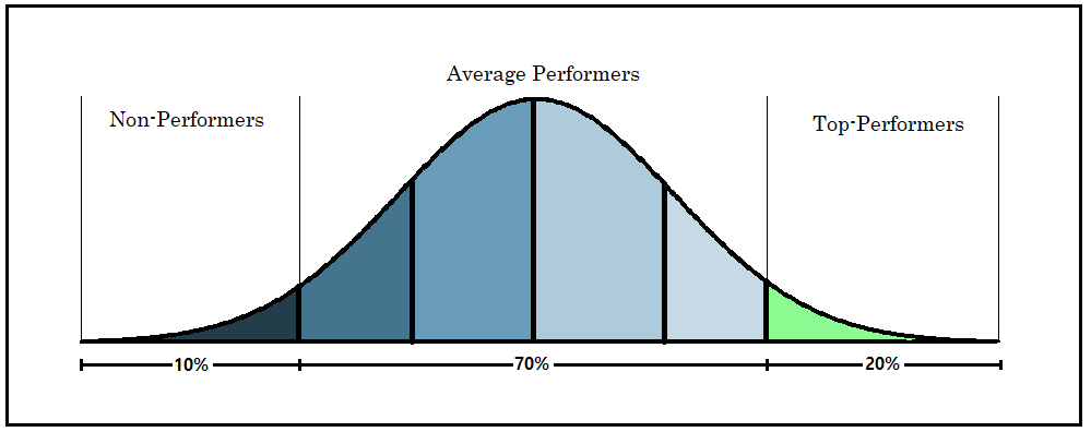
2. Most organizations use the bell curve rating system for the performance assessment of their employees in their annual performance appraisals. The bell curve method divides the employees of a company into three groups which are; high performers (top 20%), average performers (middle 70%) and non-performers (bottom 10%). This is a forced method of ranking the employees and has its own advantages and disadvantages. A graphical representation of bell curve rating system is shown in the following figure:

Family of Normal Distributions

The term normal distribution represents a family of continuous probability distributions of the same general form (bell shape) which are differed by two parameters;

1. Location parameter: defined by mean of the distribution which shows where the center of the curve is located.
2. Scale parameter: defined by standard deviation of the distribution which shows the spread of the curve or distance from the mean.

Let’s understand this concept in more detail with the help of the figure shown below; Normal distributions differ in their means (µ) and standard deviations (σ). In the above figure we have four normal distributions with means µ₁, µ₂, µ₃ & µ₄ and standard deviations σ₁, σ₂, σ₃ & σ₄ respectively. Here it can be clearly observed that;

• µ₁ = µ₃ = µ₄ > µ₂ i.e. the center of the second curve (green colored) lies before the remaining three curves on the horizontal axis of graph, thus the mean of the distribution determines the location of the center of the graph.
• σ₁ < σ₂ <σ₃ < σ₄ i.e. the spread of the fourth curve (yellow colored) is highest compared to remaining three curves. When the standard deviation is small the curve is tall and narrow (σ₁), and when the standard deviation is high the curve is short and wide (σ₄).

Properties of Normal Distribution

The normal distribution is a continuous probability distribution since the total area under the curve of a normal distribution is equal to 1. The mathematical equation for a normal distribution, also called its probability density function (pdf) is given by; Here, the parameters of this equation are as follows,

• x is a normal random variable
• µ is the mean of the distribution
• σ is the standard deviation of the distribution
• π = pi = 3.14159
• e = exponential constant = 2.7182

Following are the basic characteristics of a normal distribution;

1. It is a bell shaped continuous probability distribution, completely defined by its mean and standard deviation.
2. The area under the normal distribution curve represents probability and is equal to 1.
3. It is symmetrical about mean, each half of the distribution is a mirror image of the other half.
4. The mean, median and mode are equal due to the symmetry of the distribution.
5. The height of a normal distribution is maximum at the mean, and the height decreases as one goes from the mean towards the right tail, or towards the left tail of the distribution
6. It is a unimodal distribution i.e. having only one mode

One important property of a normal distribution is that it retains its normal shape throughout, if we apply any transformation to a normal distribution the result will also be a normal distribution, it will not change its properties. For example, the product or the sum of two normal distributions will be normal, even if we apply the Fourier Transformation to a normal distribution it will also result into a normal distribution.

What is Standard Normal Distribution & Standard Score (Z-Score)?

The standard normal distribution is a special case of normal distribution where mean is zero (µ = 0) and standard deviation is one (σ = 1) and it is abbreviated as N(0, 1). This distribution is also known as Z-distribution. Mathematically, the probability density function (pdf) of a standard normal distribution is obtained by substituting the values µ = 0 & σ = 1 in the pdf of the normal distribution discussed above in this article. Therefore the pdf of a standard normal distribution will be given by; Standardization is the process of transforming a normal distribution into a standard normal distribution, it is also called z-transformation. The normal random variable of a standard normal distribution is called as a standard score or z-score. A normal random variable can be transformed into a z-score using the following equation. Here, X is a normal random variable, µ is the mean of X and σ is the standard deviation of X.

Empirical Rule for Normal Distribution

The empirical rule of a normal distribution is also called the Three-Sigma Rule or 68-95-99.7 Rule. This is a statistical rule which states that:

• 68.27% of data lies within (+/-) one standard deviation of the mean (µ + σ)
• 95.45% of data lies within (+/-) two standard deviations of the mean (µ + 2σ)
• 99.73% of data lies within (+/-) three standard deviations of the mean (µ + 3σ)

Thus in a normal distribution, almost all observed data (99.73%) falls within three standard deviations (σ) of the mean. From the empirical rule we can conclude that, the standard deviation of a normal distribution helps us to determine the proportion of values that falls within a specified number of standard deviations from the mean. This rule also helps in assessing the normality of the data. Below is the graph of a normal curve with the Empirical Rule displayed. Please keep in mind that, a normal distribution is required to use the Empirical Rule. We cannot use this rule for skewed distributions. In the next section we will discuss the concept of skeweness in a distribution.

Skewed Distribution

Skewness is the measure of lack of symmetry of a distribution about its mean, a skewed curve appears distorted either to the left or to the right. In statistics, a distribution is called symmetric if the mean, median and mode coincide, otherwise the distribution becomes asymmetric. A distribution can be either positively skewed or negatively skewed depending upon the direction of skewness.

• If the right tail is longer we get a positively skewed distribution, here mean > median > mode.
• If the left tail is longer we get a negatively skewed distribution, here mean < median < mode.
• A symmetrical distribution will have a skewness of zero.

In a symmetrical distribution mean, median and mode are identical. More the mean moves away from the mode, the larger the asymmetry or skewness. Skewed data occurs naturally in many real life situations, for example: income distributions in almost every economy are skewed to right (or positively skewed) since a small population of very high income group people can greatly affect the mean.

Log-Normal Distribution

The log normal distribution is a transformation of normal distribution through exponentiation. A random variable X is said to be log-normally distributed if its logarithm Y = ln(X) is normally distributed, or in other words we can say if Y = ln(X) has a normal distribution, then the random variable X is said to have a log-normal distribution. Thus a random variable is said to be log-normally distributed if its logarithm is normally distributed. The lognormal distribution of a random variable X with expected value μ_X and standard deviation σ_X is abbreviated as LN(μ_X,σ_X). Log normal distributions are positively skewed distributions. All the values of a log-normal distribution X must be positive since ln(X) exists only for positive values of X. The pdf of a log-normal distribution starts at zero, increase up to its mode and decrease thereafter.

Final Words

To summarize, in this article we have discussed the concept of normal distributions, its properties and different aspects related to it. It is an imperative concept that all aspiring data scientists need to be well versed with. I hope reading this article was fruitful to you. Please let me know in the comments in case you have any queries.